
CALCULATE CheatSheet

Ajdin Burnic | Business Intelligence
2. Juli 2025
Content
- Demystify CALCULATE: Gain clarity into the inner workings of the CALCULATE function, understanding its behavior and how it affects visualizations in Power BI through a step-by-step algorithm.
- Practical Examples: Explore a series of examples of increasing complexity that demonstrate how the algorithm is applied to understand the inner workings of CALCULATE.
Table of Contents:
Introduction
Calculate is by far the most important function in DAX. At first glance, it seems intuitive and simple. However, as every DAX student knows, calculate quickly becomes anything but simple. Often the results are hard to interpret and it looks like CALCULATE either works like magic or doesn’t work at all.
This article aims to demystify CALCULATE and give you a clear algorithm that you can use in any DAX formula to correctly predict the behavior of calculate. We will present examples of increasing complexity where we use this simple yet powerful algorithm to predict the outcome of the DAX formula. Every time you feel lost, you can visit this article and check your understanding until it is solid in your mind. CALCULATE must be clearly understood to become a true DAX master. So let’s dive right in!
Fundamentals Recap
Before we begin, we’d like to mention that the terminology used in this article is based on the work of Alberto Ferrari and Marco Russo. We highly recommend that you visit their website sqlbi.com and read their books.
Now, let’s quickly review some of the basics to better understand the algorithm. If you have trouble understanding the basic elements of CALCULATE, don’t worry, it will become clearer when we get to the examples.
There are three things we should take a quick look at:
- Evaluation contexts (filter and row contexts)
- CALCULATE parameters
- Context transition
The evaluation context is the environment in which DAX formulas are executed or evaluated. In other words, DAX formulas calculate results with respect to applied filters from a visualization, such as a table or matrix visualization (filter context), and/or they are evaluated while iterating through a set of rows (row context). To always distinguish filter context from row context, you can remember the popular DAX mantra: the filter context filters, the row context iterates, they are not the same!
The special thing about CALCULATE is that it can modify the existing filter contexts or create entirely new ones, which comes in handy in many use cases. The filter context can be modified using CALCULATE parameters.
There are three types of CALCULATE parameters:
- The first is the expression that will be evaluated in the new filter context created by calculate. There is only one expression in the CALCULATE syntax.
- The second type of parameters are the CALCULATE modifiers that either remove filters (the functions with the ALL prefix; ALL, ALLEXCEPT, ALLSELECTED and ALLNOBLANKROW) or modify the relationships between tables in the model at runtime (functions such as USERELATIONSHIP and CROSSFILTERED).
- The third type of parameters are explicit filter arguments, which either overwrite the original filter context (e.g. from a visualization) using filter functions like FILTER or Boolean expressions referencing rows, or add a filter to the original one using functions like KEEPFILTERS.
The other special thing about CALCULATE is that it can transform the row context into a corresponding filter context. In other words, when CALCULATE iterates through rows, each row becomes a unique filter, meaning that each value corresponding to given columns becomes a filter on those columns. If you’re new to DAX and find this confusing, it will become clear as we explore some examples.
Finally, let’s take a look at the algorithm, which is sure to be of great value in your DAX journey.
CALCULATE Algorithm
The algorithm looks like this:
- CALCULATE evaluates its explicit filter arguments in the original filter context.
- CALCULATE makes a copy of the original filter context, which becomes the new filter context in which the expression is finally evaluated.
- If CALCULATE exists within a row context, CALCULATE performs a context transition that overwrites the original filter context, otherwise this step is skipped.
- CALCULATE applies the modifiers that remove filters or change relationships in the model.
- CALCULATE applies the explicit filter arguments to the new filter context, overwriting or adding filters to the copy of the original filter context.
Now let’s explore and analyze some examples to really solidify the understanding of CALCULATE. In the first, we’ll use the algorithm to show how CALCULATE changes the filter context by removing filters. The second example demonstrates CALCULATE by removing filters and then applying explicit filter arguments. Finally, in the third example, we’ll show how the steps in the algorithm apply when there is a row context that triggers a context transition in calcula.
Example 1
The first example is a simple scenario. We want to calculate the sales percentage of the total for different brands. To do this, we need to divide the sales amount for each brand by the total. The visual is shown below.
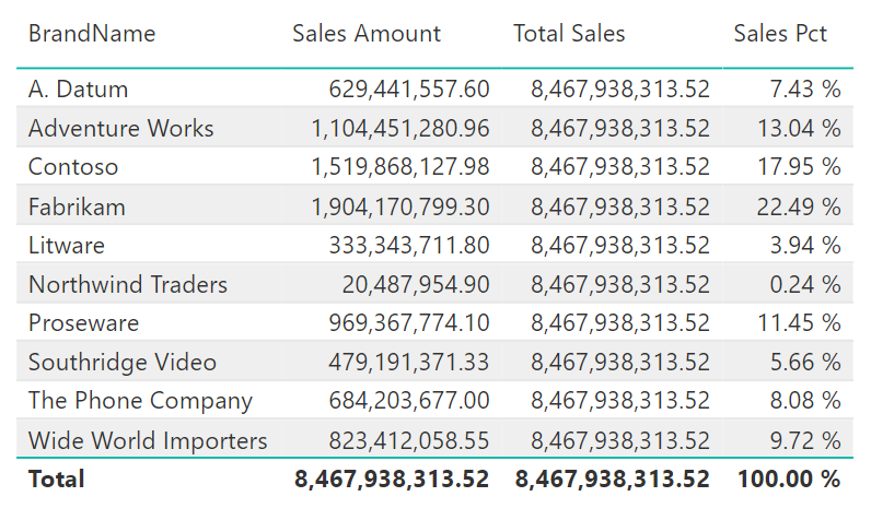
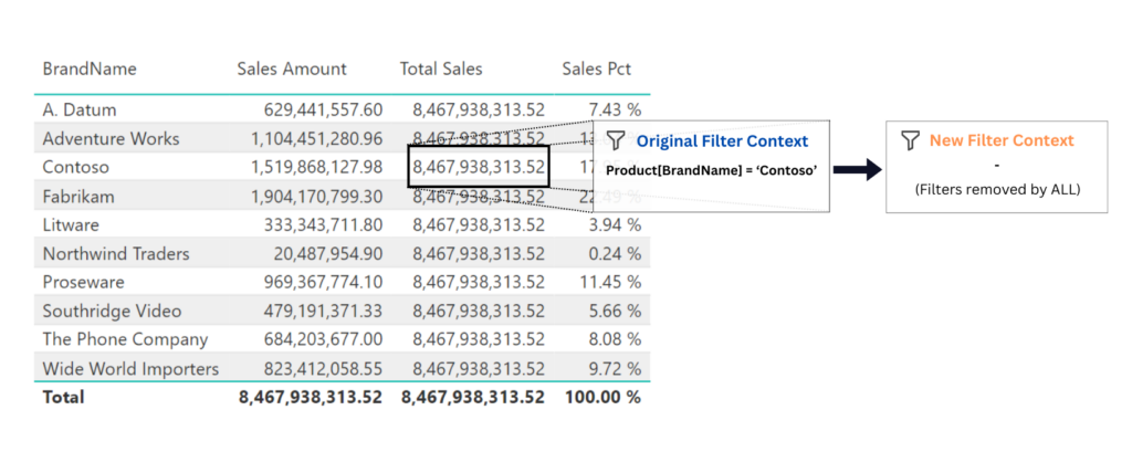
The table visual has four columns. The first column represents the brand name, which comes from the product table. The second column is the Sales Amount, which comes from the measure Sales Amount = SUMX(Sales, Sales[UnitPrice]*Sales[SalesQuantity]). The measure calculates different values for different brands because the BrandName column in the visual creates a filter context for each row. The second column is Total Sales which is presented in this visual for educational purposes. The Total Sales measure is defined as Total Sales = CALCULATE( [Sales Amount], ALL( Sales ) ). First, note that the CALCULATE function has an expression which is defined by the measure Sales Amount and a filter modifier. There are no explicit filter arguments nor is there a row context. Therefore, only steps 2 and 4 are applied. Calculate copies the original filter context and then applies the ALL filter modifier, which removes all filters on the Sales table. Now, for each cell in the Total Sales column, calculate evaluates the Sales Amount measure in the new filter context, which has no filters on the Sales table and thus the result becomes the total sales for all brands.
The Sales Pct is simply the ratio between the Sales Amount and Total Sales measures: Sales Pct = DIVIDE( [Sales Amount], [Total Sales]).
Example 2
The second example is a little more complicated. The goal is to calculate the percentage change of the sales amount for each brand with respect to the year 2011. In this scenario, we’ll first remove all filters, then reapply the filters on the BrandName and Year columns. To calculate the percentage change we need one measure that calculates the sales amount in the original filter context which is just the Sales Amount measure and one that calculates the percentage difference between the sales amount in the original filter context and the sales amount for the year 2011, regardless of which year we are in and with respect to the brand. Again, if we look at the visual below, we now see a matrix visual with rows belonging to the Product[BrandName] column and columns defined by the Calendar[Year] column.
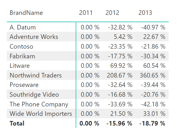
Each cell creates a filter context defined by the intersection of the year and the brand name. The solution is:
Note that in the Sales2011 variable CALCULATE has both filter modifiers and explicit filter arguments. According to the algorithm, CALCULATE evaluates the explicit filter arguments in the original filter context (step 1), which means that VALUES(Product[BrandName]) returns the row corresponding to the brand name in the visual matrix. Then, CALCULATE makes a copy of the original filter context (step 2), after which it removes all filters from the Sales table using the ALL modifier (step 4). Finally, CALCULATE applies the explicit filter arguments in which VALUES applies a filter to the BrandName and Calendar[Year] overrides the filter on the Calendar[Year] column.

Note that step 3 was skipped again because there was no row context. In the next and final example, we’ll explore a scenario where we need to create a row context that triggers a context transition in CALCULATE to solve a specific problem.
Example 3
In this scenario, we will demonstrate how context transition works and how it may be used in solving a specific problem. Imagine you want to create a table that shows the percentage of sales from only those brands that account for more than 10% of total sales. On the surface, this task doesn’t seem difficult, and it wouldn’t be if it weren’t for the total!
A first approach would probably look like:
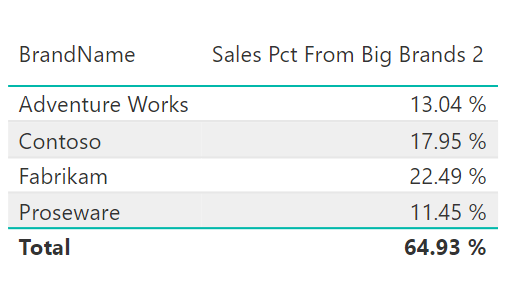
But this would produce the following visual:
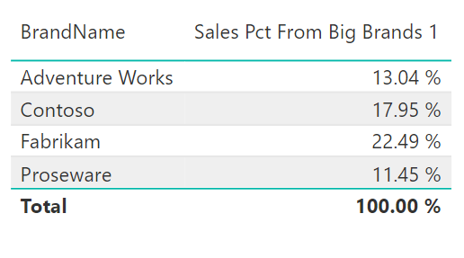
The percentages look good, but the total doesn’t add up correctly. The problem is that no filters are being applied at the total level, so the Sales Amount measure is summing up all the sales from all the brands and dividing that by all the sales again, which of course results in 100%. We need to somehow control the granularity of the summation, which means applying the same logic to each row. Now let’s have a look at the correct measure:
This measure produces the correct visual as seen below.
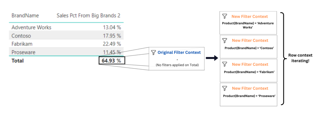
This may seem complicated at first, but it’s not. We sum over whatever VALUES produces in the original filter context VALUES creates a row context for CALCULATE. Now we finally have a situation where step 3 applies. Each row of VALUES becomes a filter for CALCULATE. So in the Contoso row, VALUES produces Product[BrandName] = „Contoso“, which then becomes the filter on the Sales table in CALCULATE. If the sales are greater than 10% of the total sales, the result is returned. What happens at the total level? Since no filters are applied on the total row, VALUES returns the entire BrandName column over which CALCULATE iterates. Each row from VALUES applies a filter to the brand name column. A value for the sales percentage is returned only if the sales percentage is greater than 10%. After completing all iterations, SUMX aggregates the results into the total, which is now correctly displayed in the visual.
Conclusion
In summary, mastering the CALCULATE function in DAX is critical to becoming proficient in Power BI and other analytical tools. By following the clear algorithm outlined in this article and exploring various examples, you can confidently navigate through different scenarios and realize the full potential of DAX formulas. Armed with this knowledge, you’ll be well-equipped to tackle various analytical challenges and gain deeper insights from your data. So dive into your DAX journey with confidence, knowing that CALCULATE is no longer a mystery, but a powerful tool at your disposal.
Download the Power BI file
By clicking the download button below, you can download the file used to write this article for free. No email or other requirements are needed.
Unterstützung rund um die Themen Finanzplanung, Unternehmensbewertung, Data Analytics, Excel und Power BI.
Walecon e.U.
Gentzgasse 148/1/5
1180 Wien
Österreich
Walecon ist Mitunterzeichner von
